Standard Isolated Digital Input
Did you know that every JNIOR since the beginning of time has used the same isolated digital input design? It is not that this design is particularly special. It is more that a better one hasn’t been suggested or required.
Here it is from external connector to the RX63N processor pin (right to left).
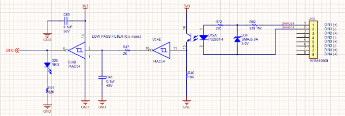
The input is optically isolated by the device U12. That means that you can bring a signal from a distance and not have to worry about it being referenced to any local GND. You won’t create any ground loop. There is no common connection between signals (they all need not be referenced to GND). To activate the input then all you have to do is turn that LED on.
The diode D34 protects the isolator LED from high voltages. You can put 30V on this input and not risk LED damage. The extra voltage above 5V is dropped across the 910 Ohm 1 Watt resistor. The input is limited by that 1W power rating. The maximum voltage is 35VDC. And 1 Watt is a lot of heat so you probably want to limit the amount of time that the input sits at that voltage.
To deal with that limitation you could add a series resistance. The maximum voltage is 5V above the square root of the series resistance assuming 1W resistors. So if you want to sense the presence of a 120VAC signal you might insert a 20K series resistance. I will leave the Ohm’s Law exercise to you. Just make sure that you can dissipate the power.
The input can be considered to have about a 1200 Ohm input impedance. It is not a high-impedance input. Therefore any signal used to drive an input must be able to deliver current into a 1200 Ohm resistance and turn on the isolation LED.
The circuit after the isolator creates a 2 KHz low-pass filter. Basically we’ve specified that input signals should not exceed 2000 Hz. The reasoning behind this lies in the need to be kind to the processor. Each input transition generates a software interrupt and executes some code. This allows JANOS to know when the state of the input changes, perform some debounce, and log the event. If this happens too fast the system can be overwhelmed having to execute interrupt code back to back and not get anything else done. That’s not ideal. So the hardware prevents it.
The processor can handle faster signals to be sure. But not if several of the inputs are cranking like that. Besides, the JNIOR is not targeted into applications that process high speed signals.
Now the RED LED that you see when the input is active is driven by the output of that filter. In other words, if the after the filter the hardware thinks that the input is ON then it turns the LED on. So those LEDs are software driven. They illuminate when the input is high enough to activate regardless of how the input is configured internally.
I’ve been meaning to see if there is a more cost-effective and compact implementation for that filter. It was implements old-school with separate gates. Works though.
The input signal then interrupts the processor. In the Series 4 each separate input has its own interrupt channel. That was not the case in the Series 3 where we had some trouble insuring that all of the input channels were properly counted when triggering simultaneously. There is no issue in the Series 4. Each input can be configured.
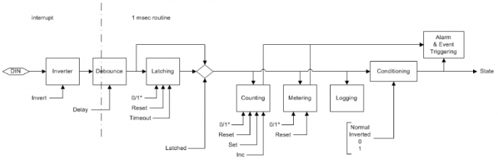
This shows the input signal processing. In this case we go from left to right. The DIN input generates interrupts. It can be optionally inverted by configuration prior to the debounce logic. This is consistent with the Series 3. Logically though you might want to invert an input afterprocessing. That inversion can be performed by the Conditioning block which finalizes the input state for the system. This is an extension in the Series 4.
The debounce delay by default is set to 200 milliseconds. Basically when an input that has been in one state for a while changes the new state is recognized immediately. The debounce timer then is started. During the delay time additional transitions restart the debounce timer and those state changes are ignored. The reported state is then refreshed once the timer does expire. The trigger is rearmed at that point.
This debounce approach effectively stretches an input pulse until it has been stable for the delay period. So if you want to detect the presence of a 60 Hz AC signal then you need to set the debounce delay long enough to ignore the time when the AC signal does not drive the input. That would be at least 17 milliseconds.
Latching

Input Latching is optional. When not enabled the function is bypassed as indicated in the flow diagram. When enabled it can be configured to latch either the HIGH or LOW state. Once latched the input state will remain the same until the input is reset. This would allow you to catch and deal with a pulse or otherwise not lose track of the fact that some alarm condition had triggered.
The latching can be configured to time out. This will latch a pulse and allow it to reset itself after a period of time. You can use this to stretch a short pulse so logic downstream has the time to detect it and to deal with it.
Counting

Once the input has been debounced and optionally latched it will be counted. The counter can be configured to count a LOW to HIGH transition (0->1) or a HIGH to LOW transition (1->0). Each counter can be reset to 0 or set to any initial value. These can even be manually incremented by an application.
When counters are displayed they can be scaled and shown with unique units. A counter can trigger an alarm when it reaches predefined values. Alarms can send email notifications.
Metering

The Usage Meter totals the length of time that an input has been active. You can tally time for the HIGH state or for the LOW state depending on configuration. Usage meters can be reset to 0. This can be useful in monitoring the operating time of a piece of equipment. An alarm can be triggered when the usage meter reaches a configured amount of time. Alarms can send email notifications. This could be helpful as a reminder for the performance of preventive maintenance.
Logging
All input and output signal transitions are by default logged. The IOLOG command can be used to review I/O activity.
Conditioning
Finally the input state can be conditioned (Series 4 only). Here the input state can be optionally inverted or forced to a HIGH (1) or LOW (0) state. The forced states may be of use in debugging applications or disabling an input without having to physically disconnect it. A forced input is masked but continues to be counted and metered.
Alarming
Note that alarms are available for Counters, Metering, and Input State. Alarms can be configured through the Registry or DCP. These can send unique email notifications.
In summary…
A digital input seems like it is a simple thing with just a HIGH or LOW input state. There is however a lot more to it. We have seen here what effect the hardware has and how the input can be configured. All of this before the input state ever affects any application.